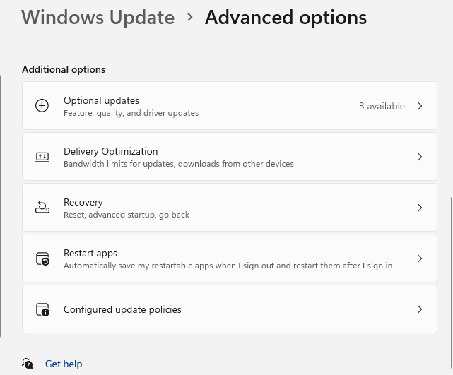
Earlier this year I had trouble connecting to the VPN on one of my devices (Windows 11 Pro 24H2). I also got this error from Teams: We Couldn’t authenticate you. This could be due to a device or network problem, or Teams could be experiencing a technical issue – Microsoft Q&A. It was an interesting learning experience, getting to see parts of the OS/networking stack in action that I don’t usually even think about. The troubleshooting process started with the usual tasks: install all Windows updates, including the optional updates. That option (from my desktop) is shown below:
The Azure VPN Client had this error message: Failure in acquiring Microsoft Entra Token: Provider Error <number>: The server or proxy was not found. Someone else ran into this issue in Azure P2S VPN Disconnecting – Microsoft Q&A. This was unusual in my case because the Access work or school pane said that I was connected.
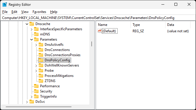
Next, we examined this registry key: HKEY_LOCAL_MACHINE\SYSTEM\CurrentControlSet\Services\Dnscache\Parameters\DnsPolicyConfig. Here is a screenshot from my desktop (not the device in question).
It turned out that there was a subkey with outdated configuration information! Deleting that subkey resolved all the connectivity issues. This was interesting to me because I assumed that general internet connectivity meant that there shouldn’t be any DNS issues whatsoever. I clearly didn’t have a good picture of how DNS is set up in these configurations and how these setups can go wrong.
Cellular networks are a ubiquitous part of modern daily life. The history of cellular technology is definitely worth knowing, even if only at the high level presented in this video on the Evolution of Mobile Standards (1G, 2G, 3G, 4G, and 5G).
Evolution of Mobile Standards [1G, 2G, 3G, 4G, 5G]
2G introduced digital modulation and came in variants like TDMA, CDMA, and GSM. 3G uses spread spectrum in the radio portion of the network whereas 4G uses Orthogonal Frequency Division Mutiplexing (OFDM). 4G also separates the user and control planes whereas they were on the same hardware in 3G (and therefore couldn’t scale independently). The following videos from Sunny Classroom are brief but helpful explanations of these communications concepts.
FHSS – Frequency Hopping Spread Spectrum
DSSS – Direct Sequence Spread Spectrum
OFDM – Orthogonal Frequency Division Multiplexing
5G offers lower end-to-end latency and higher uplink and downlink throughput than 4G because it has more bands (low, mid, and high) vs just low and high with 4G. It is also a programmable network, which lets developers access network stats via APIs.
Mobility
The discussion in the class proceeded to mobility, introducing the concept of cellular handoff, which can broadly be classified into mobile assisted and mobile controlled handover. See Handoff in Wireless Mobile Networks for more details. Another classification of types of handover is based on when the UE disconnects from one cell: hard handoff vs soft handoff. Soft handoff ensures that calls are not dropped. The professor was drawing hexagonal cells when illustrating these and I realized I had no idea why they are hexagonal. Here’s why:
antennas in a coverage area are in a hexagonal pattern… because it requires fewer cells to represent a hexagon compared to triangle or square – meaning network carriers can cover a wider area with less base stations. – The Fundamentals of Cellular System Design
An interesting aspect of the LTE packet core is that a 5G base station can be attached to it. Contrast this mode, known as 5G non-standalone to 5G standalone mode, where a 5G radio is connected to a 5G packet core. See this post on Non-standalone and Standalone: two standards-based paths to 5G for a detailed review of these modes. One advantage of the 5G packet core is that it allows for cloud-based implementations. The Boost Mobile Network, for example, is 100% implemented in the cloud. Is AWS set to flex cloud on telecom? has a discussion of such a transition (to the cloud) in the telecom space.
The antennas used on the base stations can be of multiple types, e.g. SISO and MIMO. MIMO Antennas Explained: An In-Depth Guide provides more details on the differences between these designs. A key benefit of MIMO is that it eliminates performance degradation caused by multipath wave propagation.
We also dug into the LTE and 5G network evolution, from network deployment, to network growth, then finally coverage and capacity optimization. Deployment may involve dual-radio in UEs and EPC capabilities to support interoperability with earlier generations like 2G/3G. 5G is currently in the deployment phase since 5G SA has not yet been fully rolled out. Network growth may involve cell splitting in the RAN for capacity as well as expansion of the core network. Coverage and capacity optimization may involve spectrum aggregation, advanced network topologies, and advanced antenna techniques.
The continued growth in application and device diversity, RAN complexity, and QoS variance is making networks more complex and thus harder to optimize under the current network management paradigm. Self-organizing networks (SON) were designed to address this problem. Here is an overview of SON.
3GPP SON Series: An Introduction to Self-Organizing Networks (SON)
SON is used to set many required configuration parameters when introducing a new eNB or gNB to a network e.g. IP addresses from DHCP, transmit power, beam width, supported connections, connecting to neighboring base stations via the X2 (4G) or XN (5G) connection, etc. SON can also be used for driving energy savings by shutting down carriers when less capacity is required e.g. in the middle of the night (without dropping emergency calls). Another application is coverage and capacity optimization, which involves adjusting transmission power and continuously adjusting antenna tilt to increase capacity (thus decreasing coverage) or to increase coverage (thus decreasing capacity). Mobility handover optimization is also required to avoid too early/too late handover or a ping pong between base stations. The SON architecture can be centralized, distributed, or hybrid.
5G
Finally, we took a look at 5G technology, which has much lower latencies, much higher throughput, and high capacity. Some of the key technologies I learn about include Fixed Wireless Access, in which the UE does not move, and mmWave. More info on the latter is available at What is mmWave and how does it relate to 5G? 5G also supports modified air interfaces (modified OFDM), massive MIMO, device-to-device communication, separated user and control planes, and network virtualization.
An important capability that 5G introduced is positioning, which has many potential use cases e.g. industrial, automotive, and AR/VR. See 5G positioning: What you need to know for more details. In the industrial setting, for example, 5g all in one boxes are deployed in the 5G private networks. They have a base station and a packet core in a single piece of hardware, e.g. RAK All-in-One 5G box (the first one in the search results).
The 5G core network architecture is significantly different from the LTE packet core (eNB, SGW, PGW, MME, HSS, and PCRF). It moved to a service based architecture where microservices expose functionality via APIs. This makes the 5G network programmable and extensible. This 5G System Overview covers the overall 5G architecture. These are a few of the 5G components:
Network Slice Selection Function (NSSF), which allocates slices to users
Authentication Server Function (AUSF)
Policy Control Function (PCF)
Unified Data Management (UDM), which is functionally similar to 3G and 4G’s HSS
Application Function (AF), which can let applications retrieve data like latencies
Summary
This is the final post in the Introduction to Networks series of posts. It has been an extremely enlightening course. I have appreciated how much more extensive it was than I expected from an introductory course as I try to stay on top of the fast moving tech space.
The focus of part 3 of this series is on the different types of wired networks. A key aspet of many networks is that QoS is just one concern, another key issue being how to meet guarantees for delivery of voice services. How is voice delivered? Integrated Services Digital Network (ISDN) is an international standard for voice, video, and data transmission over digital telephone or copper lines. It has two service levels. The first is Basic Rate Interface (BRI), which supports 2 bearer channels at 64kbps each and 1 D channel at 16 kbps. The second is the Primary Rate Interface (PRI), which supports 23 bearer channels (in the US) at 64 kbps each and 1 D channel at 16 kbps. The signaling/data (D) channel runs the ISDN signaling protocol based on Q.931. This video is a good high level introduction of ISDN. T1 and ISDN are used in access networks, together with technologies like IP and MPLS.
ISDN – Integrated Services Digital Network
Optical Networks
In newer generations of networks, the core is fiber (instead of copper) because it can deliver terabits per second. Installation and management of fiber networks is also much easier than copper networks. Fiber optic signals are analog – (in the infrared range).
What is the ELECTROMAGNETIC SPECTRUM
Light sources used for fiber optic communication include light-emitting diodes (LEDs), laser diodes, vertical cavity surface emitting lasers (VCSELs), Fabry-Perot lasers, and distributed feedback lasers.
How LED Works – Unravel the Mysteries of How LEDs Work!
The packet transport network is another key piece to understand. Customers send traffic to metro access, aggregation, and core portions of the network where voice and data are converged. In the packet core, wavelengths are being added and dropped by add-drop multiplexers. There are several types of ADMs with links to explanations about them from various vendors:
Open ROADM, which works to address the fact that optical systems have been proprietary (e.g. because SD FEC algorithms) on transponders are not interoperable and there are proprietary control loops between transponders and other optical components).
The next video gave me a better understanding of customer concerns with ROADMs and FOADMs.
Tutorial: To ROADM or Not to ROADM: When does a FOADM make sense in your optical network?
Other major types of network components include amplifiers, regenerators, and equalization nodes. Transponders map client side signals to wavelengths for high speed transport. They can be contained in a field-replaceable unit (FRU). Common types of pluggable optics include SFP+ (Small Form-factor Pluggable), CFP4, and QSFP28. Amplification is an analog process of boosting signal strength and is done in the optical domain (no conversion to electrical). Any impairments in the signal are boosted as well. A single pump laser is used for this. Regeneration can reshape and retime the optical signal but requires conversion to the electrical domain then back to the optical domain, making it more expensive to implement.
How a Fiber Laser Works
Major types of amplifiers in optical networks include EDFA (Erbium Doped Fiber Amplifer), Raman amplifier, and Hybrid Raman-EDFA amplifier. These are great explanations of these amplifiers:
Working Principle of Erbium Doped Fiber Amplifier (EDFA)
The EDFA – how it was developed.
Wavelength Selective Switch (WSS) was first implemented using MEMS but did’t work well because the hinges would fail. Liquid Crystal on Silicon (LCoS) is now commonly used to implement WSS since it has no moving parts. It can also support Flexgrid.
What is LCoS Based Wavelength Selective Switch – FO4SALE.COM
Optical patch panels are another component in fiber networks. They are used to join optical fibers where a connect/disconnect capability is required.
Handling Failure
There are 2 types of protection in networks:
Network protection: ensures that customer SLAs are met by preventing failures. Optical protection examples include mesh restoration (GMPLS, SDN), SNCP (OTN), UPSR & BLSR for SONET, and 1+1 or 1:1 circuits (active vs inactive backup circuit). Packet protection examples include MPLS fast reroute, LAG, G.8031, G.8032.
Equipment protection: focuses on protecting individual nodes.
I couldn’t emphasize this enough: this is such a broad field with so many technologies! What an introduction to networking!
The previous post introduced different types of networks and some of their architectural details. In this post, we look at the biggest problem network engineers work on: congestion. How are networks designed to address it? The professor starts tackling this area with a discussion of Quality of Service (QoS). Quality is defined in terms of the underlying requirements e.g. throughput, delay, jitter, packet loss, service availability, and per-flow sequence preservation. Services can be best effort, or other classes like gold service. Cisco’s Quality of Service (QoS) document discusses four levels of metal policy (platinum, gold, silver, and bronze), for example.
Class of Service (CoS) is a traffic classification that enables different actions to be taken on individual classes of traffic. Contrast this to type of service (ToS), which is a specific field in the IPv4 header (used to implement CoS). Juniper Networks post on Understanding Class of Service (CoS) Profiles equates QoS and CoS, but the professor explains that QoS is a more abstract concept than CoS.
QoS is a set of actions that the network takes to deliver the right delay, throughput, etc. QoS timeframes affect the way congestion is handled. For example, scheduling and dropping techniques and per-hop queuing are useful for the low millisecond time regime common in web traffic. Congestion over hundreds of milliseconds typically affects TCP (e.g. round trip times, closed-loop feedback) and this is addressed via methods like active queue management (AQM) and congestion control techniques like random early detection (RED). Congestion that occurs in the tens of seconds to minutes range is addressed by capacity planning.
How is QoS achieved in the data and control planes? By queuing, scheduling, policing, and dropping. The roles of the data and control planes are quite extensive as per the router diagram used to describe them. This is without getting into the details of the management plane e.g. the element management systems (per node) and the network management systems they communicate with. Control plane QoS mechanisms handle admission control and resource reservation and are typically implemented in software. Resource Reservation Protocol (RSVP) is the protocol mostly used in practice for control plane QoS. There are many explanations on RSVP, e.g. this Introduction to RSVP and this RSVP Overview. The primary QoS architectures are integrated services (Intserv) and differentiated services (Diffserv). Intserv uses RSVP and although it doesn’t scale, it is useful when guaranteed service is required.
We start a deep dive into the QoS techniques with queuing. There are different types of queues: first come first served (FCFS/FIFO), priority queues, and weighted queues. Packet schedulers can have a mix of these approches, e.g. 1 priority queue and N other weighted queues. Performance modeling can be done on queues. For voice traffic, the distribution of the arrival rate of traffic is a Poisson distribution. Therefore, the delay of packets and the length of the queue can be accurately modeled/predicted! See M/M/1 queues as a starting point (M/M/1 is Kendall notation and is more fully described in the next video).
Queuing Theory Tutorial – Queues/Lines, Characteristics, Kendall Notation, M/M/1 Queues
Data Plane QoS Mechanisms
These data plane QoS mechanisms are applied at each network node: classification, marking, policing and shaping, prioritization, minimum rate assurance. Below are more details about each.
Classification
This is the process of identifying flows of packets and grouping individual traffic flows into aggregated streams such that actions can be applied to those flow streams. Up to this point, I have had a vague idea of what a flow is but not a proper definition. The instructor defines a flow as a 5-tuple of source & destination IP addresses and TCP/UDP ports and a transport protocol. What is a Network Traffic Flow? discusses various ways of defining a flow, and this is just one of many. Classification needs to avoid fragmentation because the 5-tuple information is only in the first packet. There are 4 ways of classifying traffic:
Simple classification – the use of fields designed for QoS classification in IP headers e.g. the type of service (TOS) byte in IPv4. There are complications with using the DTRM bits of the TOS (e.g. minimizing delay and maximizing throughput could conflict).
Implicit classification – done without inspecting packet header or content, e.g. by examining layer 1 or 2 identifiers.
Complex classification – using fields not designed for QoS classification or layer 2 criteria like MAC addresses.
This is simply setting the fields assigned for QoS classification in IP packet headers (DSCP field) or MPLS packet headers (EXP field).
Source marking is applied at the source of the packets
Ingress marking: used when source cannot mark correctly or cannot be trusted to do so.
Rate Enforcement
This is done to avoid congestion. Policing is a mechanism to ensure that a traffic stream does not exceed a defined maximum rate. It stands in constrast to shaping, which is typically accomplished by queuing (delays traffic, never drops it). One type of policer is the token bucket policer. It never delays traffic and cannot reorder or reprioritize traffic. See Cisco’s Policing and Shaping Overview and QoS Policing documents for details. This is one of the rate limiting algorithms discussed in the video below (I found this video’s explanation more intuitive).
Five Rate Limiting Algorithms ~ Key Concepts in System Design
The next stage is prioritization of the traffic. 4 possible approaches: with prioritiy queues, e.g. where VoIP traffic always has highest priority, other queues can be starved by the scheduler. Weighted round robbin will take more packets from the high priority queues but still cycle through the other queues, taking fewer packets from them. Weighted bandwidth scheduling considers the packet sizes instead of just packet counts per queue (e.g. just taking 1 packet from a low priority queue can have negative impact if the packet is huge). Deficit round robbin is the one used in practice. It keeps track of the history of the number of packets services, and not just instantaneous values. I found the next video to expand on these brief explanations of scheduling algorithms.
How Do Schedulers in Routers Work? Understanding RR, WRR, WFQ, and DRR Through Simple Examples
One of the points that came up in discussion was that the schedulers use Run-to-completion scheduling, which means that a packet must be fully processed before starting on another packet. Routers have an interface FIFO (Tx buffer) on the physical link. When it fills up, this signals to the scheduler that there may be congestion downstream, thereby allowing for back pressure flow control. There is also multi-level strict policy queuing which allows for multiple priority queues instead of just 1 (e.g. voice & video) but not as common today.
Routers also drop packets to prevent unacceptable delays caused by buffering too many packets. There are different dropping strategies, e.g. tail dropping (dropping from the back of the queue), weighted tail dropping (>1 queue limit via heuristics), and head dropping (rare).
Active queue management (AQM) is a congestion avoidance technique. It works by detecting congestion before queues overflow. These are some techniques for AQM:
These QoS mechanisms operate in the context of an overriding architecture, integrated services (Intserv) or differentiated services (Diffserv). IntServ can be used in the financial industry or medical health facilities, for example. These are delay sensitive applications where unbounded scaling is not a real requirement. IntServ explicitly manages bandwidth resources on a per flow basis. DiffServ was developed to support (as the name suggests) differentiated treatment of packets in large scale environments. It does this using a 6-bit differentiated services code point (DSCP) in the IPv4 ToS header or the IPv6 traffic class octet. Classification and conditioning happen at the edge of the DiffServ domain. Actions are performed on behavior aggregates (contrast this to the per flow actions of IntServ). The next technology we learn about is Multiprotocol Label Switching, defined as follows on Wikipedia:
MPLS is similar to IntServ in that it lets you define an end-to-end path through the network for traffic but without reserving resources. It is a hop by hop forwarding mechanism, which stands in contrast to IP which works by making next hop routing decisions without regard to the end-to-end path taken by the packets. MPLS can be deployed on any layer 2 technology (multiprotocol). Benefits of MPLS include fast rerouting in case of failures and providing QoS support. One of the settings in which MPLS is used is in SD-WAN. This article provides a helpful contrast: What is the difference between SD-WAN and MPLS? These are the main applications of MPLS:
Traffic Engineering: allows network administrator to make the path deterministic (normal hop-by-hop routing is not). In other words, a frame forwarding policy can be used instead of relying on dynamic routing protocols.
QoS: the MPLS EXP bits are used for marking traffic per the labels.
This is quite the array of topics, especially for an introduction to networks course. I have a greater appreciation of how broad this space is.
I’m taking an online introductory course on networks. I have been surprised by how much ground this course is covering. I didn’t expect to cover wireless (mobile) networks, for example. I looked for videos on some of the topics to learn more, e.g. 4g network architecture – YouTube. Networking is turning out to be much cooler and more interesting than I thought possible. This post is a compilation of all the key topics introduced in the course (in the general order they were introduced, but not particularly organized into a coherent story).
My main takeaway from this first video is that 4G networks are entirely packet switched (basic, but new to me).
4G LTE Network Architecture Simplified
The next video on how messages are transmitted to the cell phone tower is insightful as well. I appreciated the high-level discussion of antennas.
How WiFi and Cell Phones Work | Wireless Communication Explained
The concept of control plane and data plane came up as well. One advantage of this separation as per the overview below are independent evolution and development of each (e.g. control software can be upgraded without changing the hardware).
M2.1: Overview of Control and Data Plane Separation
5G Service Based Architecture | Telecoms Bytes – Mpirical
Then of course there are the fundamental concepts of throughput, delay, and packet loss error. Jim Kurose’s book (and video below) covers these topics but it’s been a while since I read that book.
The professor also clarified the difference between bandwidth and throughput. The next video briefly touches on this distinction:
The course has also introduced me to the concept of spectral efficiency as part of understanding the difference between bandwidth and throughput. There is no shortage of concepts to learn about, from the different types of lines like T1 and T3 to bit robbing to the existence of network interface devices. The video below is good intro to T1.
DS1 (T1) Fundamentals
There was also a discussion about cable networks, with an onslaught of concepts like Hybrid fiber-coaxial. This Cable 101 video is a helpful resource.
The HFC Cable Systems Introduction video below starts out with a comparison of coax and fiber then explains the flow of signals from the core network to the home.
HFC Cable Systems Introduction
I still need to learn more information about the Cable modem termination system (CMTS) and the next resource is perfect. It mentions CMTS vendors like Arris, Cisco, and Motorola, which inspires me to look up the Cisco CMTS.
Cable Modem Termination System Tutorial (CMTS)
I have never researched how most of these systems work so I am greatly appreciating this introduction to networks course! Here’s a video on how cable modems work, including their interactions with the CMTS.
How Cable Modems Work
The communication between the CMTS and the CMs is done via DOCSIS. Here is the reference I found with insight into DOCSIS.
DOCSIS® 3.1 – An Overview
Something I picked up is that CableLabs does a lot of the research for these systems. Other concepts to know include wavelength-division multiplexing (WDM), which was used in the traditional coax networks. The following explanation is an example of WDM in fiber.
Next, we get into the 7-layer OSI model. The example given for the physical layer is SONET technology. Another foray into T1 technology reveals the fact that bipolar transmission is used for T1 since it is more power efficient.
Multiplexing is the next interesting topic introduced. I have included some videos below on the different types of multiplexing employed in communications.
FDM involves modulating message signals over carrier frequencies then using bandpass filters to extract the individual signals.
The course also addresses transmission fundamentals like the difference between bit rate and baud rate, the Shannon–Hartley theorem, the Nyquist–Shannon sampling theorem, modulation, modems, and codecs. I have compiled a few videos covering these topics below.
Here is an explanation of the Shannon–Hartley theorem:
Channel Capacity by Shannon-Hartley | Basics, Proof & Maximum Bandwidth Condition
We then start getting into network addressing. One of the important concepts here is how the exhaustion of IPv4 addresses is handled: private IP addresses, DHCP, subnetting, and IPv6. One particularly interesting point was the difference between IPv4 and IPv6 headers:
In a discussion of the impact of TCP on throughput, the professor called out TCP global synchronization as an issue that networks need to avoid. Here’s one video about it.
Avoiding packet reordering is another important aspect of TCP. The contrast with UDP is especially interesting when other protocols like Google’s QUIC are designed. The RTP protocol (a relative of UDP, informally speaking) is used for VoIP. This is a good description of RTP:
One of the security podcasts I listened to mentioned using tcpdump to analyze traffic. It looks like a tool you need to build for yourself since is no download page. Build instructions are well documented at tcpdump/doc/README.windows.md. This post is a summary of all the instructions required, including for installation of the Npcap: Windows Packet Capture Library & Driver. First get the Npcap SDK:
cd /c/repos
git clone https://github.com/the-tcpdump-group/tcpdump
cd tcpdump
mkdir build
Run these commands from the Developer command prompt:
cd \repos\tcpdump\build
cmake "-DPCAP_ROOT=C:\software\npcap" -G "Visual Studio 16 2019" -A x64 C:\repos\tcpdump
msbuild /m /nologo /p:Configuration=Debug tcpdump.sln
This takes only 40 seconds on my desktop. Next, run the Npcap 1.79 installer to ensure that launching tcpdump does not fail with this error: “The code execution cannot proceed because wpcap.dll was not found. Reinstalling the program may fix this problem.” We can now run tcpdump:
cd Debug
tcpdump.exe
When tcpdump starts up, it indicates that it is listening on a given device.
C:\repos\tcpdump\build\Debug> tcpdump.exe
tcpdump.exe: verbose output suppressed, use -v[v]... for full protocol decode
listening on \Device\NPF_{SOME-GUID}, link-type EN10MB (Ethernet), snapshot length 262144 bytes
Interestingly, the repo does not have much (any?) documentation on how to use tcpdump. However, there are links to tutorials and numerous other resources at Home | TCPDUMP & LIBPCAP. As per the repo:
Richard Stevens gives an excellent treatment of the Internet protocols in his book “TCP/IP Illustrated, Volume 1”. If you want to learn more about tcpdump and how to interpret its output, pick up this book.
The earlier test tcpdump did not display any traffic on my desktop. Following an introduction to using tcpdump at the Linux command line | Opensource.com, list the available devices using tcpdump -D then select one of them and pass it as the --interface argument. This allows me to find the device that with network traffic.
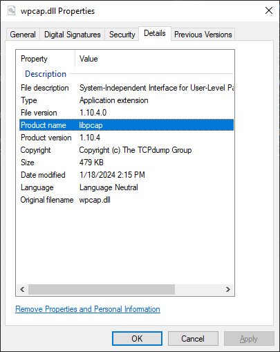
How does tcpdump -D generate the list of network devices? The main function of the application detects the -D option then calls the show_devices_and_exit function, which in turn retrieves the devices by calling the pcap_findalldevs function. Stepping into this call reveals that it is in C:\Windows\System32\wpcap.dll. As shown in the properties of wpcap.dll below, it is part of the libpcap product. This explains why tcpdump fails to start if the Npcap installer is not executed (when “wpcap.dll was not found”). I’m interested in the actual enumeration of network devices but that appears to be part of libpcap, specifically pcap.c. I’ll save that exploration for another day.